
By Nick Chambers
Last week, we covered how distribution of redds influences habitat capacity. Now, we look into how scientists and managers most commonly estimate if harvest is appropriate for a certain population and at what level. This is generally done with modeling, which is nothing more than taking all of the data that is available for a certain population and combining it with a little bit of math and a few assumptions.
The model is capable of estimating different population parameters, such as growth rate and the inflection point at which the data begins to show effects of density dependence. However, as with any modeling exercise, the quality of the outcome is wholly dependent on the quality of data it relies on. The right kind of data with a good model can provide meaningful estimates and insights, but if the model is based on very limited data and large assumptions, there is much greater uncertainty about the estimates, and in the worst case, the results could completely mischaracterize the status and trends of a population.
It’s also important to remember the classic quote: “All models are wrong, some are just more useful.” This is because models are inherently a simplification of natural processes. It’s impossible to collect all types of information across all locations, times and times in the life cycle of a fish.
There are many types of models, but the stock-recruit model is the most widely used for estimating escapement goals and harvest levels.
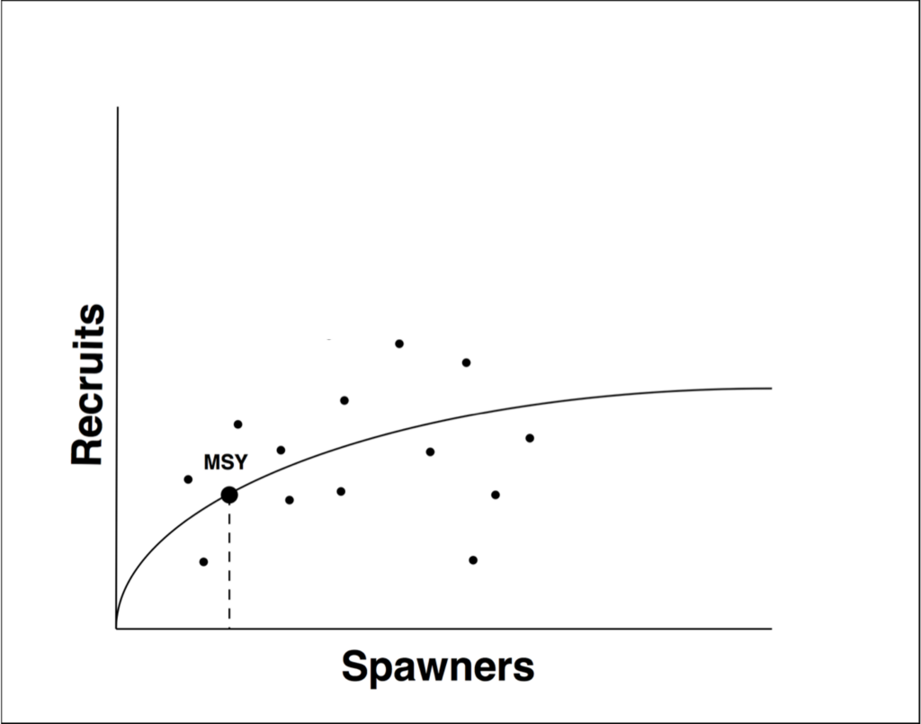
A Stock-Recruit Model is an equation that compares the number of adults that spawned to the number of offspring that survive to “recruit” into the next generation. The general assumption is that the number of offspring produced by a cohort of adults is proportional, suggesting that when abundance is very low, there is compensation owing to a low density of competitors. Alternatively, when abundance is high, there is a proportional reduction in survival of offspring owing to density dependence processes.
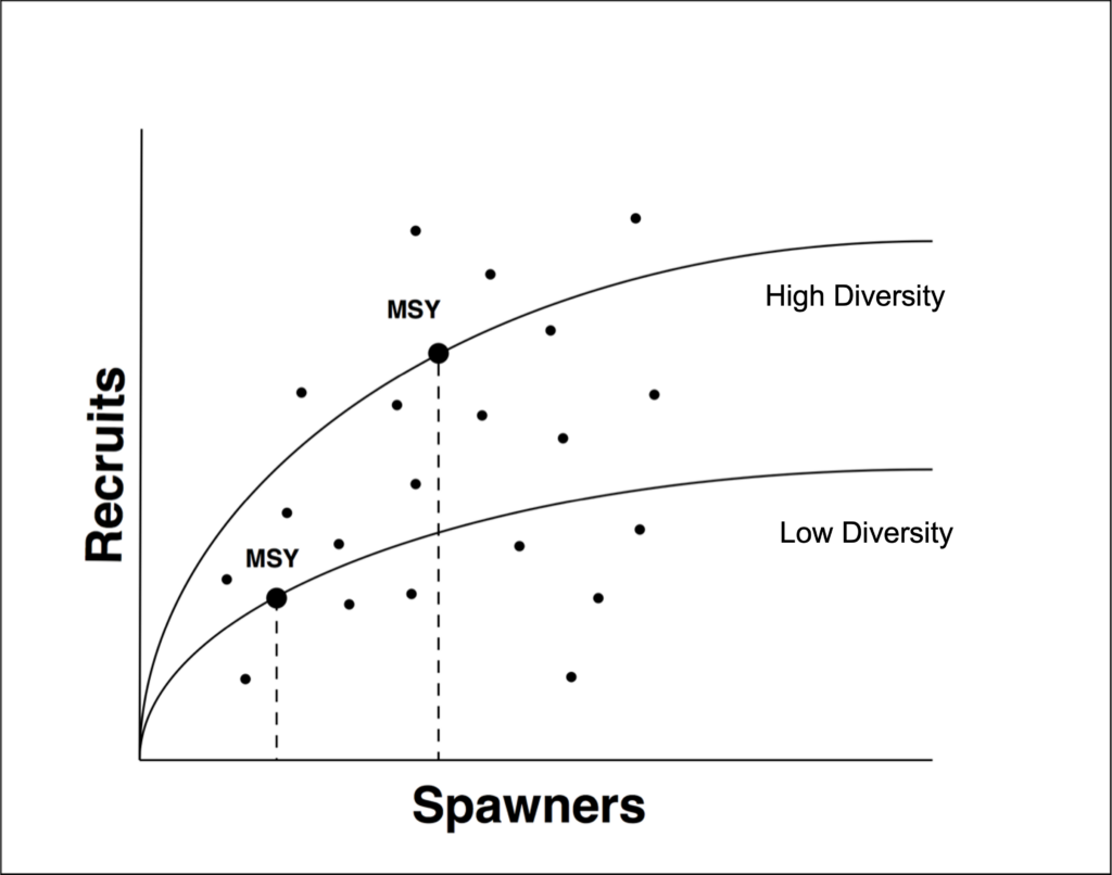
These types of models are often used to analyze and estimate the productivity of a population of fish and how it varies through time. Productivity differs from abundance in that abundance is simply how many fish you have at any one time, while productivity is X number of fish produced Y number of fish. By graphing productivity of a population over many generations, scientists can — with sufficiently detailed data — estimate how many fish it takes to fill up or “seed” the available habitat. In years with very high escapements we may see a proportionately lower productivity due to increased competition among juveniles. That increased competition results in fewer offspring from each parent surviving, so the productivity is lower. Conversely, in years with lower run sizes there is less competition and the population may be more productive due to higher juvenile survival. At that point, the model is presumably estimating the effects of density dependence and how those effects change at different densities.
As discussed last week, populations can theoretically compensate for the effects of harvest because reduced abundance will lead to increased productivity, as long as we meet a minimum escapement goal. This seems like a simple and elegant system right? Well, unfortunately it gets a bit more complicated when looking at the bigger picture.
In reality, density dependence, as measured by changes in growth and/or mortality in relation to the number of individuals in a certain area, is essentially ever present. In fact, density dependence is generally strongest at low densities!
Sounds weird right?
Well, remember that territory size increases, as density decreases. Think of the stream as a conveyor at a sushi restaurant, it is much easier to defend the prime spot where you get your pick of dishes from one or two competitors rather than 10, 20 or 50 competitors. Fish farmers have long known this, which is one reason they always aim for an optimum (and surprisingly high) density because there is less territorial behavior at high densities.
Now, let’s look at some real world examples.
Bristol Bay sockeye salmon are one of the most famous and well known salmon fisheries in the world, and their management has been based on extensive monitoring and research. Sockeye in Bristol Bay support average harvest rates of 50% or more, and the populations have actually increased since the beginning of the large commercial fishery in the 1970’s. 2021 even saw the highest run size ever recorded. However, Bristol Bay sockeye are showing reductions in age and size at maturity, which is common in fisheries and often what scientists refer to as “fisheries induced evolution.”
It is not clear how the change in size and age, which is also likely linked to climate change, will affect the population’s resilience. For now, Bristol Bay provides a good example of where a population (consisting of many smaller stocks) is compensating for harvest. Likely due to data collection taking place before populations were subject to intensive harvest.
Unfortunately, there are no examples like Bristol Bay for steelhead, where data was collected and a stock-recruit model was fit to a relatively intact population. Even in places like Washington’s Olympic Peninsula (OP), where there is a long-term and extensive data set, the populations were subject to intensive fisheries for long periods before formal data collection and modeling began. Unfortunately, OP winter steelhead populations are at an all time low, despite most watersheds having a large part of their land base in pristine condition inside the Olympic National Park. OP steelhead experience the highest known harvest rates of any wild steelhead populations in the country. It’s easy to hypothesize that the decline of OP winter steelhead is partly related to the long history of intensive fishing; although that is not clear from the stock-recruit models, which suggest there is little risk associated with the current harvest levels. So why is management in Bristol Bay having more success than winter steelhead on the OP?
There are several plausible explanations.
First, the OP watersheds are not entirely pristine. High quality habitat is the foundation for strong runs of salmon and steelhead and Bristol Bay remains essentially as it was 200 years ago.
Second, while habitat is important, it is also possible that the biology of steelhead, such as their complex suite of life histories, makes them more difficult to model and manage. A life history is the series of life stages that an individual undergoes to reach adulthood. For example, steelhead spend one to five years (or more) in freshwater and one to four or more years in saltwater, while some even remain in freshwater their entire lives as rainbow trout. Each combination of years spent in fresh and saltwater would be a different life history, or a different strategy taken to reach sexual maturity.
Enumerating the number of life histories is one way to measure diversity within a population or species. Steelhead have a much more diverse set of life histories when compared to salmon. For instance, pink salmon have the least with one or two life histories, while sockeye and chum average about three to five and chinook and coho display about five to fifteen. Scientists have recorded up to 38 life histories in a single population of steelhead, which is the most among salmonids. And of course, resident rainbow trout may spawn with and produce steelhead.
It is easier to model and manage a species with a simpler set of life histories because nearly all fish have a similar age class. As age classes become more complex, it makes it more difficult to derive clean linkages between adults and juveniles. While all species display a few life histories that are more common than others, steelhead have a wide array of age classes that are only displayed by a few fish, and only likely to contribute significantly to production in occasional years when conditions are just right. Simply, a life history model for steelhead is more complex and difficult to manage than a model for pink salmon. Further, it also means that when fisheries harvest pink salmon, the harvested fish will be replaced by an individual with the same life history (see caveat in next paragraph). For a diverse species like steelhead, it is relatively easy to reduce the frequency, even eliminate, rarer and less common life histories, which can result in simplification of the population. It is therefore possible that life histories have been reduced on the OP prior to the onset of modern monitoring and research programs, which in turn could bias assumptions made in the stock-recruit models.
Third, diversity is not only about age classes, and even species with simpler life histories display more variability than one might think. For instance, although pink salmon exhibit minimal diversity in terms of age classes, they do display diversity in entry-and spawn-timing. Researchers in Alaska found that small differences in pink salmon spawn timing of one month actually increased the productivity of a population in Auke Creek, in Juneau, Alaska. The bimodal spawn timing was helpful because juveniles emerged from the gravel across a broader range of time than if all individuals had spawned together. And juveniles from early-spawning adults dispersed further from the redd, creating a void for later-emerging juveniles. Basically, staggering the time at which fry emerged from the gravel reduced competition between the early and late emerging individuals.
To be fair, pink salmon have almost no freshwater residence time as juveniles, meaning there may have been little opportunity for competition between these two groups of juveniles to begin with. Still, similar results were found for juvenile steelhead in an experiment by Ted Bjornn in Idaho in the 1980s, though the ultimate effects remain unclear because it was experimental and the juveniles were not tracked through adulthood. Regardless, if a stock-recruit model is based on a highly altered population, it will provide results based on the attributes of that modified population, and without historical data preceding fisheries, it is very difficult — if not impossible — to determine how much productivity has been potentially lost to to changes in the biological structure of the population.
In summary, the best managed fisheries combine rigorous data collection with statistically robust modeling. Unfortunately, unlike Bristol Bay, data on steelhead is often limited to the recent past. This requires us to make assumptions, and pretty big ones in regions where recent data is sparse — such as the Southern Oregon Coast. If we assume that the current population attributes are the same as the historical attributes, we are likely underestimating their diversity and potential productivity. For example, did steelhead spawn over a broader period historically than they do now? Did they stagger the use of habitats? Are they occupying all the available habitats?
While some diversity has been lost to habitat degradation, especially in rivers with impassable dams, fisheries also exert strong influences, and there is substantial evidence that fisheries can alter size, age classes and even spawn and entry timing. And this is why it is essential to evaluate stock-recruit models with care. They are often based, especially for steelhead, on an extensive set of assumptions that are rarely tested and they have a difficult time dealing with a large number of life histories, including contributions from resident rainbow trout and repeat spawners. Additionally, historical data preceding intensive harvest is almost always lacking.
This is not to say results from stock-recruit models are always incorrect for steelhead. Rather, it depends on the quality and length of the data set, and it’s important to be skeptical, because reduced productivity could be conflated with reduced diversity.
Next week, we will explore this topic of how life history diversity relates to estimating habitat capacity.